Introduction
Most people assume a supermarket chain has a price.
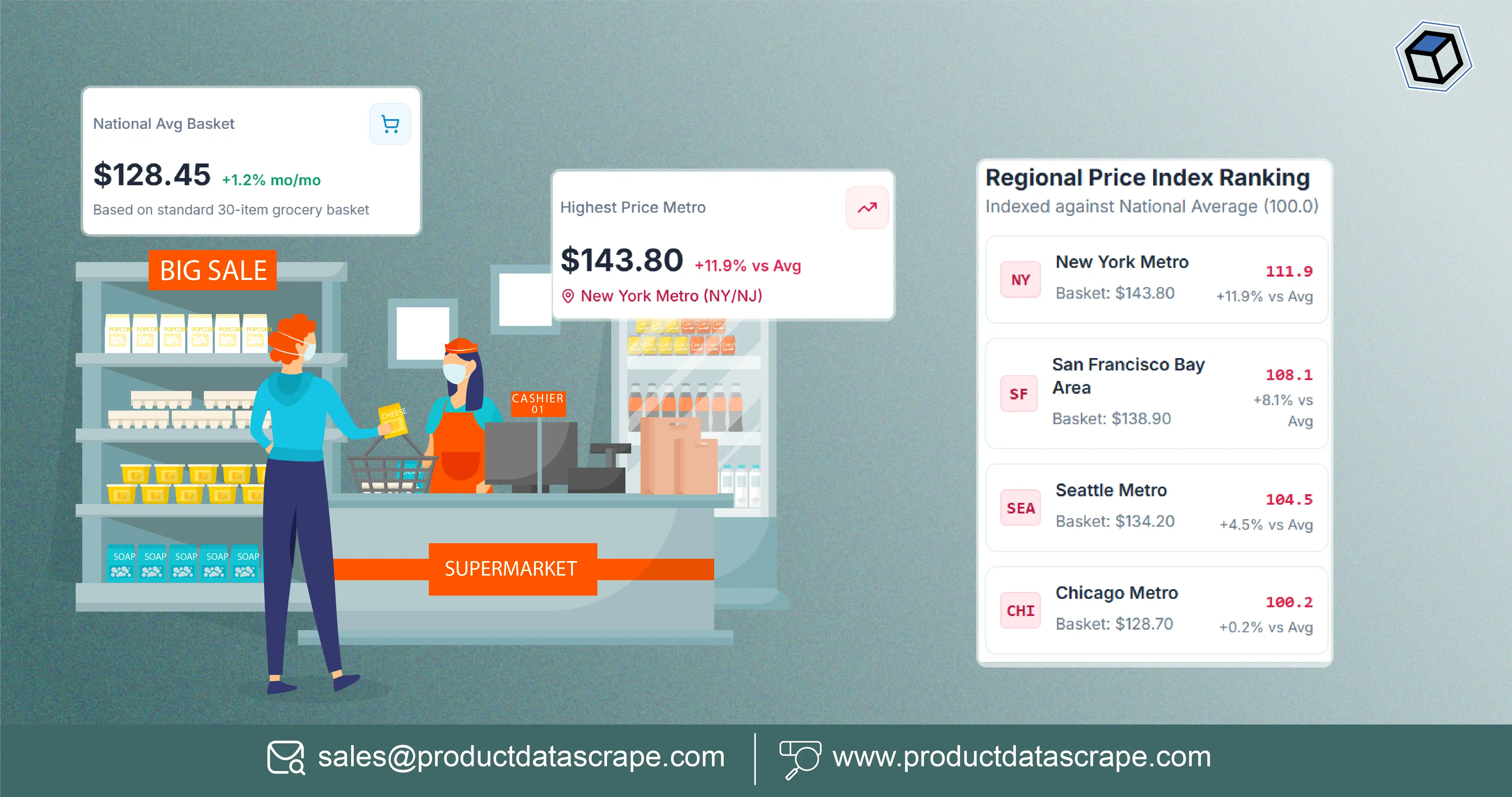
It has many. The same banner, the same SKU, the same day — and a different shelf price in a metro store than in a suburban one, in one state than in another, in a dense urban delivery zone than in a peripheral one. This is not unusual or hidden. It is ordinary retail practice, in the United States and India alike, and it is entirely visible in public listing data if you capture at the right granularity.
What is not visible is why. And the gap between measuring regional price variation and explaining it is where most analysis of this data goes wrong — usually in a direction that is confident, quotable, and unsupported.
This guide covers how to run regional price data extraction properly, what it reliably shows, what it cannot show, and how the difference between those two things determines whether the analysis is useful or merely provocative.
Why a Single Chain Runs Many Prices
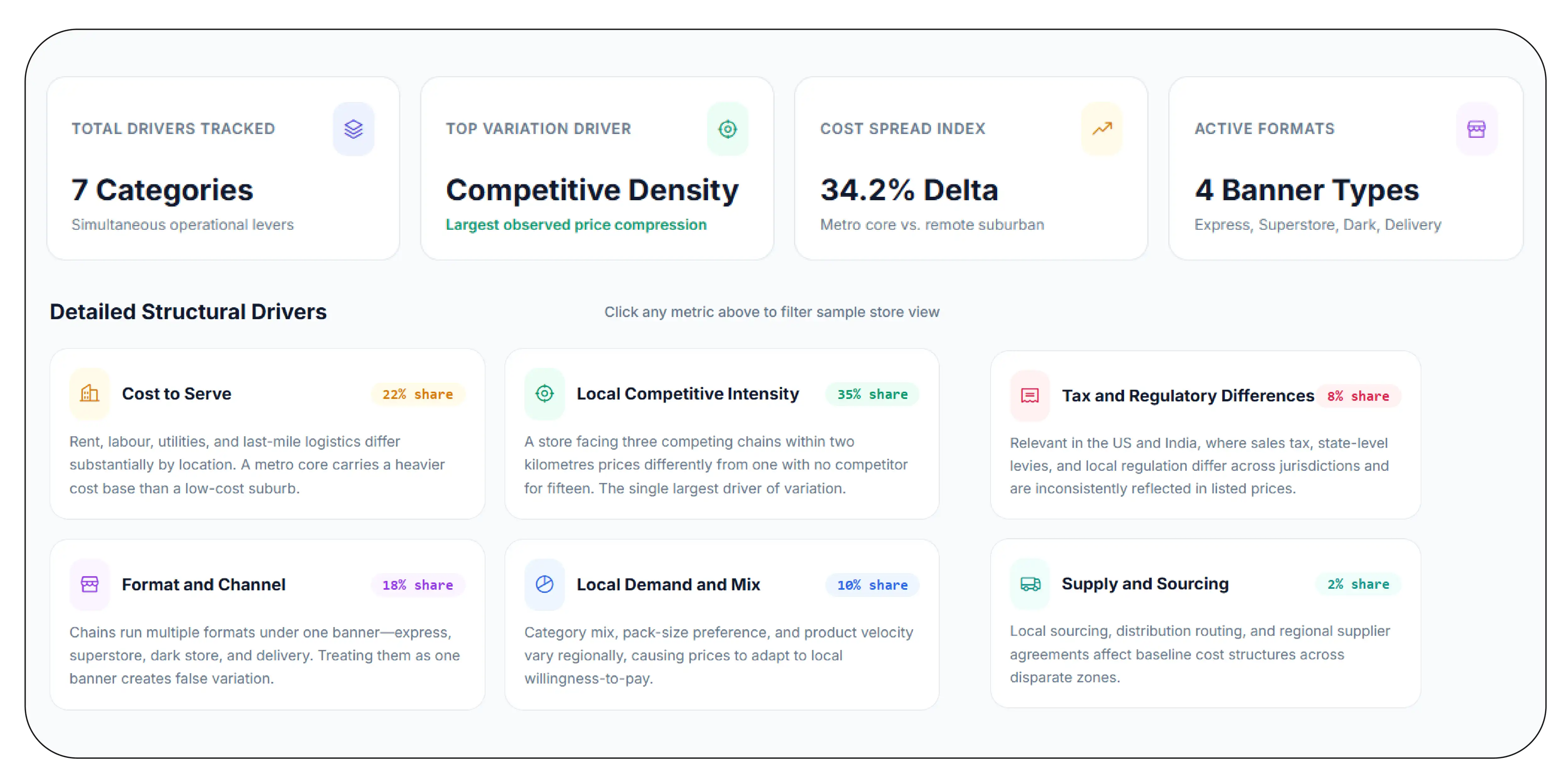
Before measuring, it helps to know what plausibly produces the variation, because the list is longer than most analyses assume.
Cost to serve. Rent, labour, utilities, and last-mile logistics differ substantially by location. A store in a high-rent metro core carries a different cost base than one in a low-cost suburb, and a delivery zone at the edge of a distribution network costs more to reach than one beside the depot.
Local competitive intensity. A store facing three competing chains within two kilometres prices differently from one with no competitor for fifteen. This is often the single largest driver of observed variation, and it is measurable — variation tends to compress where competition is dense.
Format and channel. Chains run multiple formats under one banner — express and superstore, dark store and full store, in-store and delivery. These are frequently priced as separate propositions, and treating them as one banner produces variation that is really format difference.
Local demand and mix. Category mix, pack-size preference, and product velocity vary regionally, and prices follow.
Tax and regulatory differences. Particularly relevant in both the United States and India, where sales tax, state-level levies, and local regulation differ across jurisdictions and are sometimes reflected in listed prices and sometimes not — which is itself a measurement problem, discussed below.
Promotional calendars. Regional promotions run on different schedules. A snapshot comparison across regions frequently measures promotion timing rather than base price.
Supply and sourcing. Local sourcing, distribution routing, and regional supplier agreements affect cost.
Any of these can produce the variation you observe. Several usually do, simultaneously. That is the central analytical fact about this dataset, and the reason the most common interpretation error is so tempting.
The Interpretation Trap
Regional price data extraction produces a very attractive headline: the same chain charges more in some places than others. From there it is a short step to attributing the difference to a single cause — most commonly, that certain areas are charged more because of who lives there.
Price data alone cannot support that step, and treating it as though it can is both an analytical error and a reputational risk.
Here is the problem in concrete terms. Suppose you observe that stores in lower-income postal codes carry higher prices for a matched basket. That observation is consistent with several very different explanations:
- Those locations have lower competitive density, so prices are less compressed
- Those locations are served by a smaller-format store, which is a different cost structure and often a different price list
- Those locations sit further from distribution infrastructure, raising cost to serve
- The store mix in those areas skews toward formats with structurally higher prices
- Some combination of all of these
And it is also consistent with a pricing policy that differentiates on local demographics. The point is not that the last explanation is wrong. It is that price data cannot distinguish it from the others, because all of them produce the same observable pattern.
A rigorous analysis therefore does two things. It reports the variation precisely — magnitude, geography, category, and persistence. And it states explicitly what the data does and does not identify, listing the plausible drivers rather than selecting one. Where a causal claim is genuinely wanted, it requires additional data the price feed does not contain: store format, competitive density, cost-to-serve proxies, and ideally the retailer's own stated policy.
Product Data Scrape supplies the measurement. Causal attribution belongs to the analyst, with the additional evidence required to support it — and, where the conclusion is publishable and consequential, with legal review.
Getting the Measurement Right
Regional price variation is easy to measure badly, and a badly measured version produces variation that is real in the spreadsheet and absent in the world.
Capture at location granularity, not at brand level
A national price feed for a chain is an average or a default. Regional variation requires capture at the level the price actually varies — store, zip code, pincode, or delivery zone. If your capture does not carry a location identifier on every record, you cannot measure this at all.
Match the SKU exactly, including pack size
This is where most analyses silently break. Chains stock different pack sizes in different formats and regions — a 900 ml bottle in one store, a 1 litre in another. Comparing them as "the same product" produces an apparent price difference that is entirely a size difference.
Every comparison must be normalised to a unit — per kilogram, per litre, per 100 grams, per unit count — and the raw pack size retained so the normalisation can be audited.
Capture simultaneously
Prices move. Comparing a price captured in one region on Tuesday with another captured on Thursday measures the calendar, not the geography. Regional comparison requires captures within a tight window.
Separate base price from promotion
A regional promotion produces a price difference that is real but temporary and structurally different from a base-price difference. Both matter. Conflating them makes the analysis unstable — run it a week later and the conclusion reverses.
Handle tax presentation consistently
In the United States, listed prices commonly exclude sales tax, which varies by jurisdiction — meaning the listed price understates the checkout difference between locations. In India, listed prices typically include applicable tax. Either convention is fine; mixing them within one analysis, or failing to state which you used, is not.
Distinguish assortment from price
If a SKU is absent in one region, that is an assortment fact, not a price fact. Excluding unavailable SKUs from a basket comparison, without saying so, silently changes what the basket measures.
Sample Data: One SKU, Five Locations
An illustrative same-day capture of a single grocery SKU across five locations of one chain.
| Location |
Format |
Pack size |
Listed price |
Price per litre |
Promotion active |
vs national median |
| Metro core A |
Express |
900 ml |
89 |
98.9 |
No |
+12% |
| Metro suburb B |
Superstore |
1 L |
92 |
92.0 |
No |
+4% |
| Tier-2 city C |
Superstore |
1 L |
85 |
85.0 |
No |
−4% |
| Tier-2 city D |
Superstore |
1 L |
79 |
79.0 |
Yes |
−11% |
| Peripheral zone E |
Dark store |
900 ml |
95 |
105.6 |
No |
+19% |
Illustrative figures.
Three things in this table are worth pulling out, because each is a trap.
The two highest per-litre prices are both 900 ml packs. Compared on listed price, the gap between location A (89) and location C (85) looks like 4 rupees. Compared per litre, it is nearly 14 — because A is a smaller pack. Without unit normalisation, the analysis understates the real variation and misidentifies which location is most expensive.
Location D is cheapest because of an active promotion, not because of a lower base price. Include it in a base-price analysis and the conclusion about regional structure is wrong.
Locations A and E are different formats — express and dark store — which are frequently priced as separate propositions. Whether they belong in a like-for-like comparison with superstores is a methodological decision that has to be made explicitly, not by accident.
The structured record:
{
  "chain_id": "chain_a",
  "product_id": "GROC-OIL-SUNFLOWER",
  "captured_at": "2026-07-15T11:00:00+05:30",
  "capture_window_minutes": 45,

  "location": {
    "location_id": "IN-400001",
    "location_type": "pincode",
    "store_format": "express",
    "region": "metro_core"
  },

  "pack": {
    "size_value": 900,
    "size_unit": "ml"
  },

  "pricing": {
    "listed_price": 89,
    "base_price": 89,
    "promotion_active": false,
    "promotion_type": null,
    "price_per_litre": 98.9,
    "tax_treatment": "inclusive"
  },

  "availability_state": "in_stock",

  "context": {
    "national_median_price_per_litre": 88.3,
    "variation_vs_national_median_pct": 12.0
  }
}
Note capture_window_minutes and tax_treatment. Neither is glamorous. Both are the difference between a dataset that survives scrutiny and one that does not.
What the Aggregate Data Reliably Shows
With the methodology right, several patterns hold up consistently.
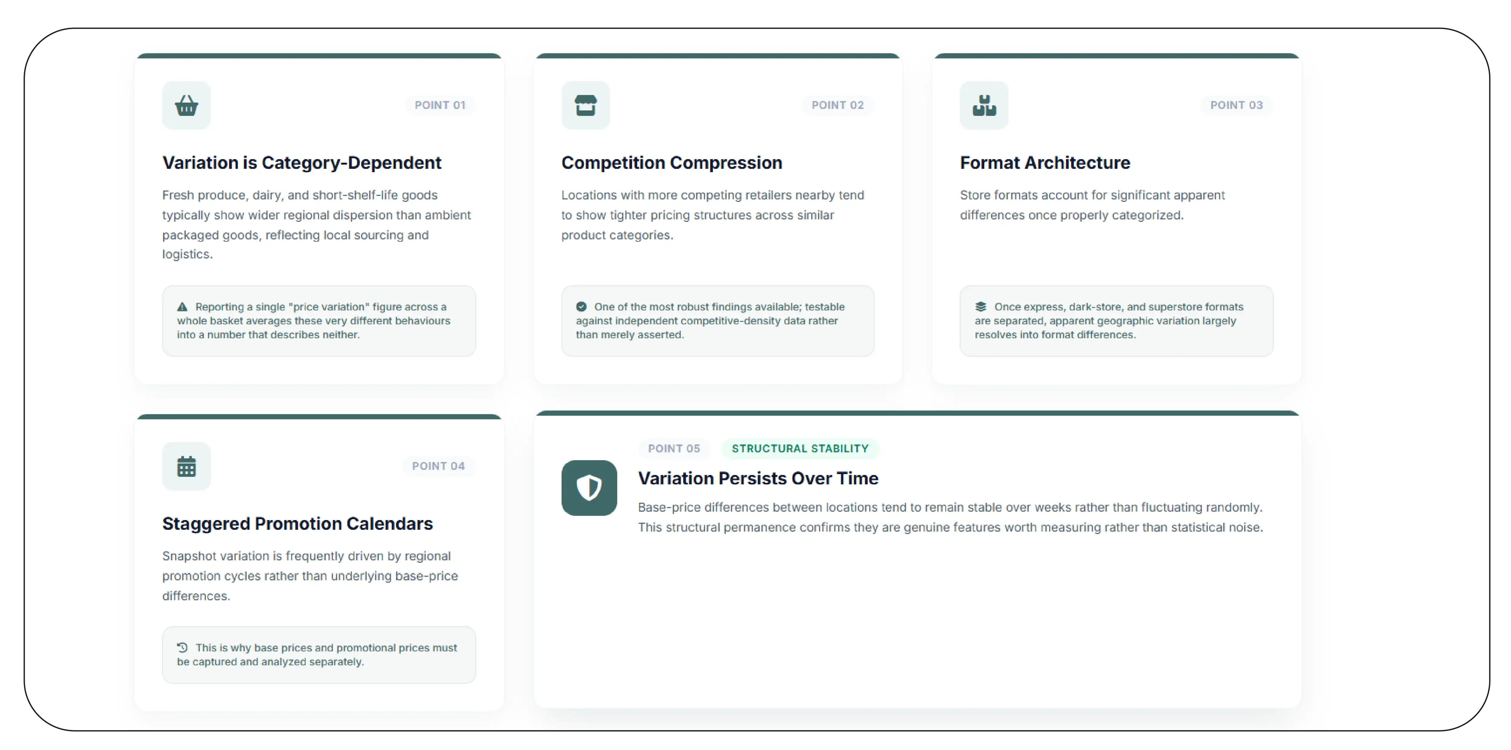
Variation is category-dependent. Fresh produce, dairy, and short-shelf-life goods typically show wider regional dispersion than ambient packaged goods, reflecting local sourcing and logistics. Reporting a single "price variation" figure across a whole basket averages these very different behaviours into a number that describes neither.
Variation compresses where competition is dense. Locations with more competing retailers nearby tend to show tighter pricing. This is one of the more robust findings available from this data, and — usefully — it is testable against independent competitive-density data rather than merely asserted.
Format explains a large share of variation. Once express, dark-store, and superstore formats are separated, a substantial portion of apparent geographic variation resolves into format differences.
Promotional timing is regionally staggered. A meaningful share of snapshot variation is promotion calendar rather than base-price structure, which is why base and promotional prices must be captured separately.
Variation persists. Base-price differences between locations tend to be stable over weeks rather than fluctuating randomly — which is what makes them a structural feature worth measuring rather than noise.
Who Uses Regional Price Data Extraction
FMCG brands discover that their product sells at meaningfully different prices across a single retail partner's estate, which affects volume forecasting, trade investment allocation, and how promotional funding is deployed regionally.
Pricing and category teams at retailers benchmark their own regional structure against competitors' — visible only through location-level external capture.
Economists and inflation researchers use location-level price data as an input to price-index and dispersion work, where geographic granularity is the entire point and methodological transparency is non-negotiable.
Public-interest and consumer researchers study price accessibility across geographies — work that is valuable precisely when it is careful about the causal limits described earlier.
Investors and analysts track regional pricing behaviour as a signal of competitive pressure in specific markets.
Frequently Asked Questions
Can you capture prices at zip code or pincode level?
Yes. Location-level capture is the requirement for this analysis, and every record carries its location identifier and store format where available.
How do you handle different pack sizes across regions?
Every price is normalised to a unit — per litre, per kilogram, per 100 grams — with the raw pack size retained so the normalisation can be checked.
Can you separate promotional from base prices?
Yes, and it is essential. A promotion-inclusive regional comparison measures the promotional calendar as much as the price structure.
Does this show why prices differ?
No. It shows precisely that they differ, by how much, where, in which categories, and how persistently. Explaining the difference requires additional data — format, competitive density, cost-to-serve — which we can help structure but which price data alone does not contain.
How many locations can be monitored?
As many as the analysis requires. Coverage design — which locations, at what density — is part of the engagement, because a poorly designed location panel produces a precise answer to the wrong question.
Measure Carefully, Claim Carefully
Regional price variation is one of the most interesting datasets in retail and one of the easiest to over-interpret. The variation is real, it is substantial, and it is fully visible in public data captured at the right granularity. The explanation is not visible, and the distance between "we observed this" and "this is why" is where credibility is won or lost.
The analyses that hold up are the ones that measure precisely — unit-normalised, simultaneously captured, format-separated, promotion-separated — and then say exactly what the measurement supports and no more. That discipline is not a limitation on the work. It is what makes the work usable by a pricing team, a regulator, a journal, or a court.
Product Data Scrape delivers regional price data extraction across supermarket chains in the United States, India, and other markets: location-level capture with store format, unit-price normalisation with raw pack size retained, simultaneous multi-location capture windows, base and promotional price separation, documented tax treatment, and availability state on every record.
Delivered as JSON, CSV, via REST API, or pushed to your warehouse — with methodology documentation designed for analyses that will be published, challenged, or acted on commercially.
Ask us to design a location panel for your question. We will tell you what the data can settle, and what it cannot.
Product Data Scrape — turning marketplace complexity into decision-ready data.


 Singapore
 EMAIL
EMAIL
 PHONE
PHONE


.webp)
.webp "thumb")
.webp "thumb")
.webp "thumb")










.webp)